Learning effects lead to path dependency
First Posted: 2021.05.22, Last Revised: 2021.05.22, Author: Tom Brown
- Learning effects lead to path dependency
- Including learning in your model => many distinct local optima
- => Diverse choice of low-cost future energy systems
- Can't just look at one
Conclusions from Niclas Mattsson's pioneering work in 1990s:
Learning by modeling energy systems (PhD thesis, 2019)
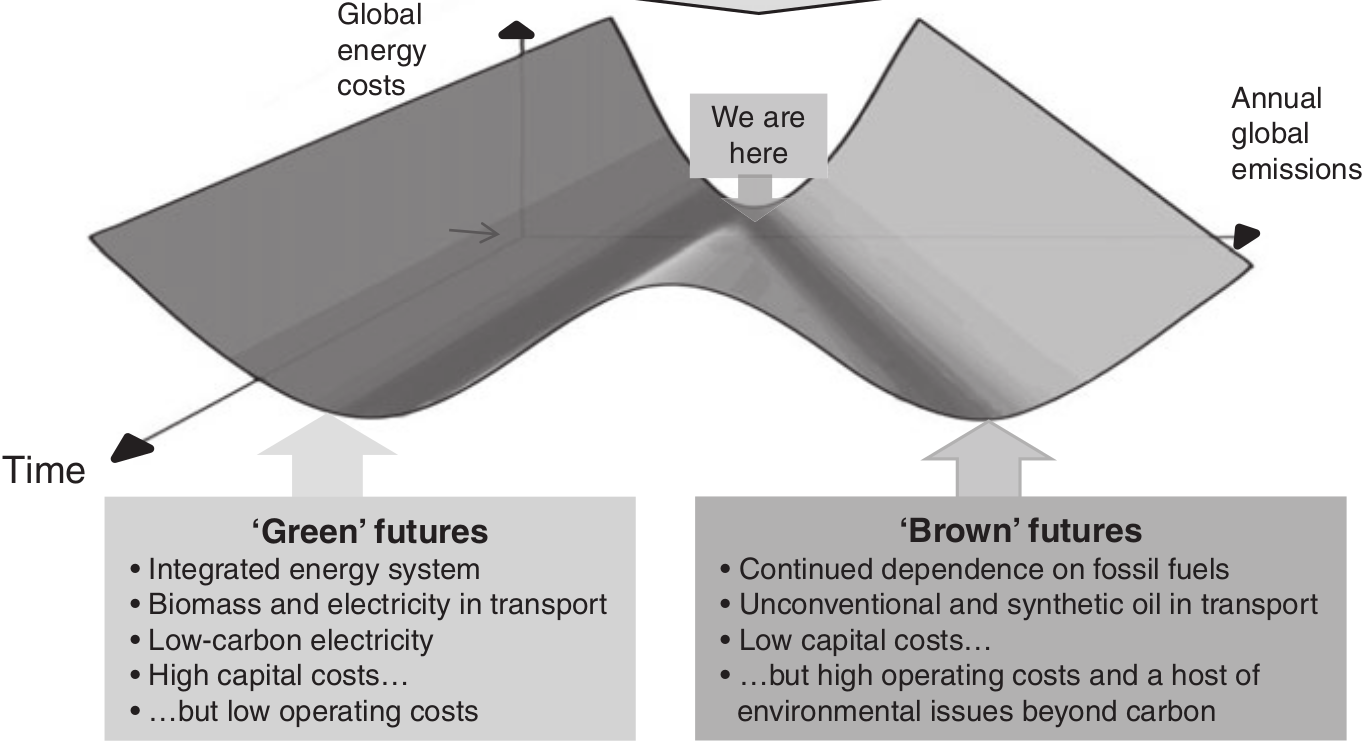
Figure 1: Source: Planetary Economics by Michael Grubb et al, 2014
—
So what did Niclas do?
He ran an energy model with built-in learning curves and showed that with exactly the same model (same equations, all same data inputs, costs, etc.) you can get radically different energy pathways with similar total costs:
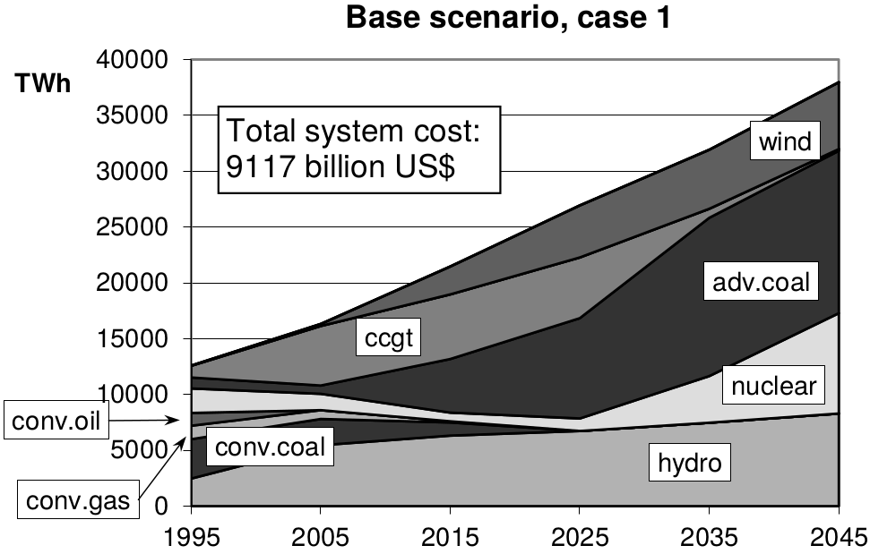
Figure 2: Source: Mattsson, 2019
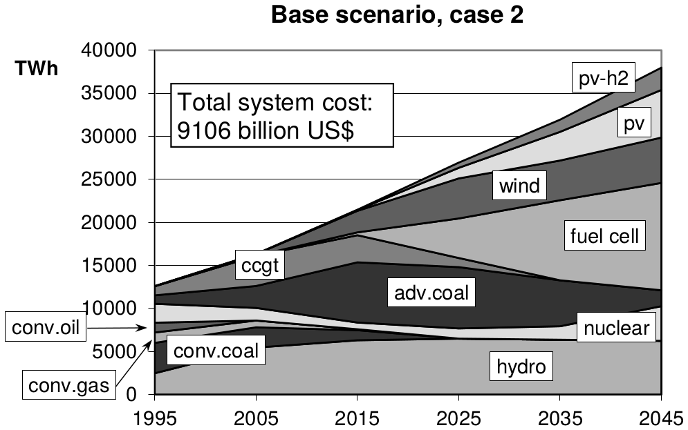
Figure 3: Source: Mattsson, 2019
—
Case 1 is coal-heavy while Case 2 has lots of PV. They cost roughly the same.
Case 2 is different because large investments get triggered early for PV and other technologies, which take them down the learning curve, saving costs later in the simulation:
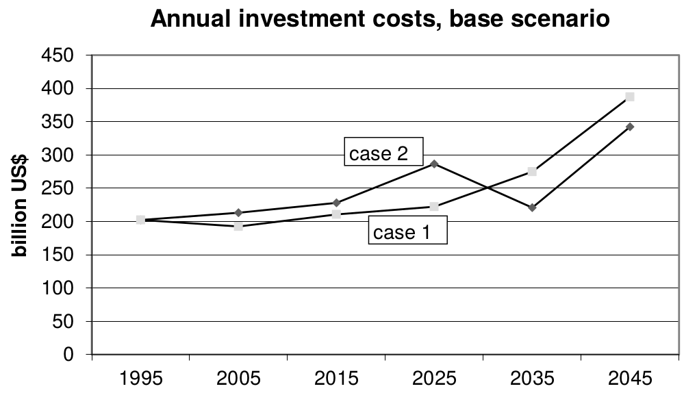
Figure 4: Source: Mattsson, 2019
—
This phenomenon, that technology investments and learning now can save costs later, was well understood by the fathers of the German renewable subsidies programmes, Hermann Scheer and Hans-Josef Fell, which brought down the costs of PV.
—
How can the same model deliver such different results?
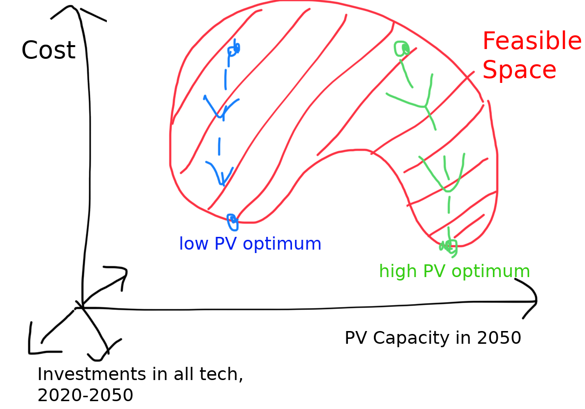
Because learning curves introduce non-convexities into the optimisation.
This leads to local optima in the solution space.
Depending on where the solver starts looking (green/blue), you end up in different optima:
—
If the solver starts its search on the left and looks for decreasing cost, it lands at the blue low-PV, high-coal optimum.
If it starts on the right, it lands in the green high-PV optimum.
It's hard to build solvers to find these different solutions, so they're often ignored.
—
This diversity often goes unacknowledged in the energy modelling world where models that have endogenous learning curves aren't used to explore all solutions. (Please correct me if I'm wrong.)
—
Policy-wise, this general phenomenon of path dependency shows how we can choose (within limits) how we steer our technology investment towards solutions that society wants (e.g. high acceptance, high co-benefits, etc.).
—
Conclusion: there are lots of different possible low-cost low-emission energy systems out there, depending on which technologies we choose to invest in.
—
Now for some more technical details.
This is NOT the same as the near-optimal solutions that crop up in the Method to Generate Alternatives, since those solutions are convexly connected to the global optimum. Here we're talking about far-away distinct near-optimal solutions.
—
Niclas has some comments on this:
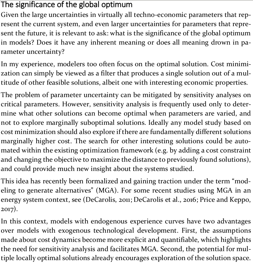
Figure 5: Source: Mattsson, 2019
—
What about models that approximate the non-linear learning curves with a piecewise linearisation to turn it into a MILP? (A technique Niclas co-invented with Sabine Messner)
Niclas has a trick to find the local optima by forcing constraints and seeing if they become non-binding:
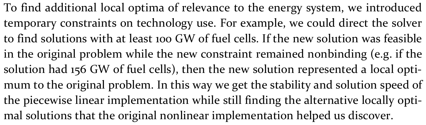
Figure 6: Source: Mattsson, 2019